Pipeline Tour

This page shows the full video-to-inverse-dynamics workflow as a sequence of inspectable stages. The images below are generated from the package APIs themselves: vis_2d(), vis_3d(), StorageResult.plot(), estimate_grf(), and the exported Three.js visualizer. The pose and visualizer frames use the same trial instant: t = 13.86 s.

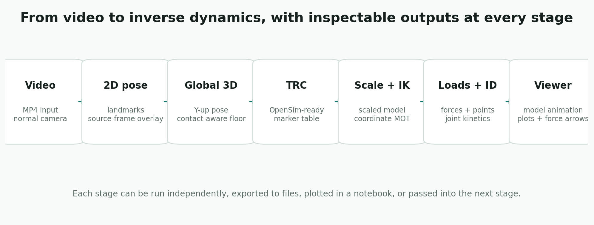
Stage 1: 2D Pose On The Image

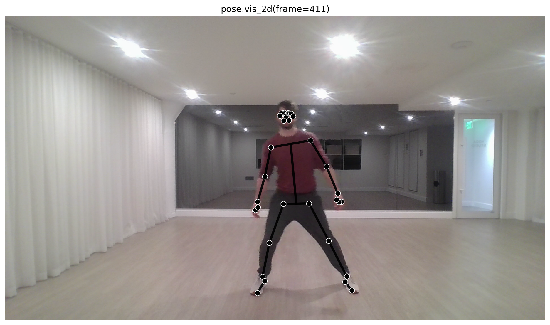
The first check is visual. pose.vis_2d() draws the 2D landmarks and body connections directly on the source frame so tracking quality is easy to judge.

pose = mm.estimate_pose("data/subject01.mp4", root_centered=False, floored=True)
pose.vis_2d(frame=411)

Stage 2: Root-Centered 3D Pose

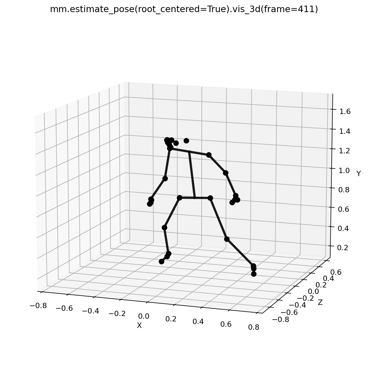
Root-centered 3D pose is useful for inspecting the body shape and motion without camera placement. It keeps the pose centered around the pelvis, which makes early pose issues easier to see.

root_pose = mm.estimate_pose(
    "data/subject01.mp4",
    root_centered=True,
    floored=True,
)

root_pose.vis_3d(frame=411)

Stage 3: Global Pose After PnP And Flooring

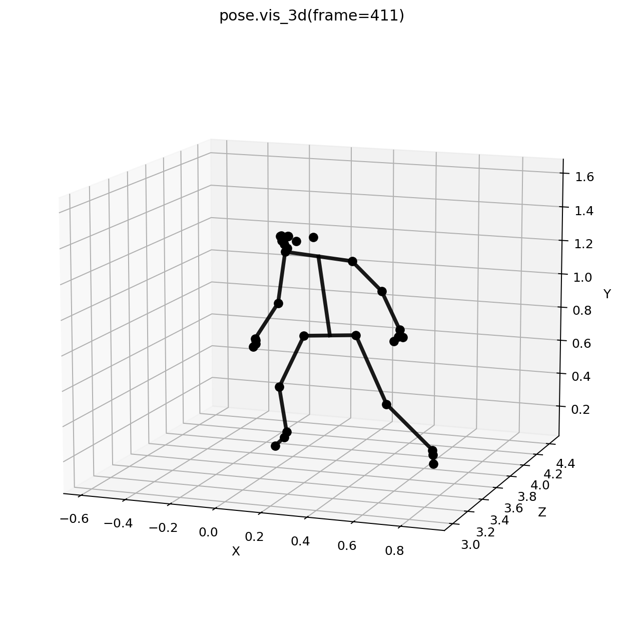
The global pose uses 2D-to-3D PnP placement and contact-aware floor estimation. This is the pose you usually export to TRC for OpenSim.

pose = mm.estimate_pose(
    "data/subject01.mp4",
    root_centered=False,
    floored=True,
)

print(pose.metadata["translation_method"])
print(pose.metadata["floor_method"])
pose.vis_3d(frame=411)

Stage 4: Key IK Angle Signals

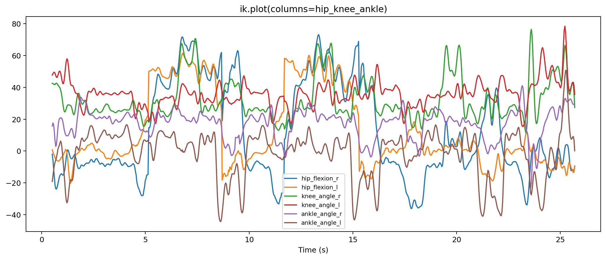
After scaling and IK, the output is an OpenSim coordinate .mot file. The signal sheet below is produced with ik.plot(...) and focuses on the key angles most people check first: hip, knee, and ankle motion.

scaled_model = mm.run_scaling(pose, model="pose")
ik = mm.run_ik(scaled_model, backend="fast")

ik.plot(columns=[
    "hip_flexion_r", "hip_flexion_l",
    "knee_angle_r", "knee_angle_l",
    "ankle_angle_r", "ankle_angle_l",
])
ik.to_dataframe()

Stage 5: Key Estimated Forces

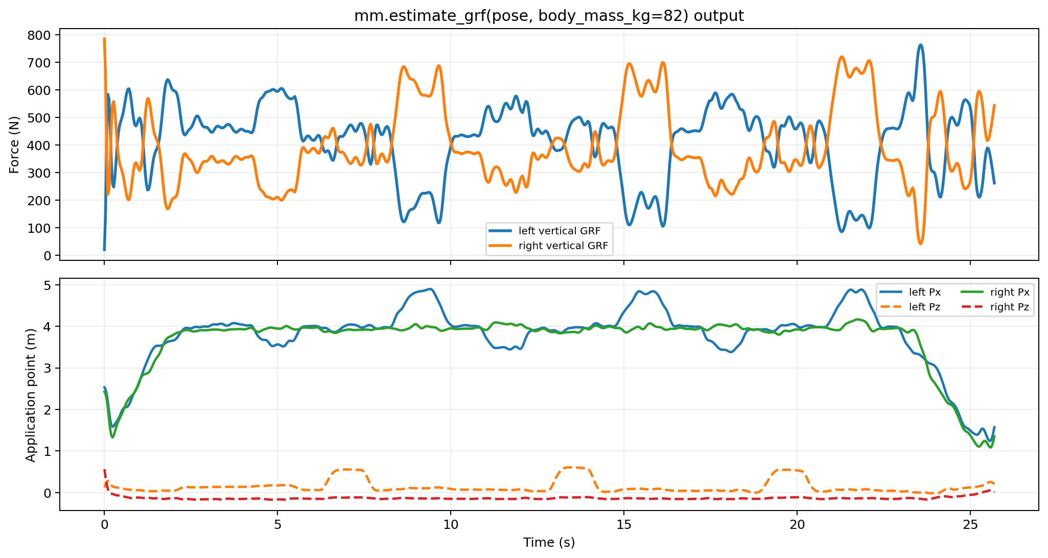
Estimated ground-reaction forces are returned as external-load specs and then written as OpenSim external-load signals. The sheet is built from mm.estimate_grf(...).to_dataframe() and highlights vertical support and center-of-pressure placement, which are the first checks before inverse dynamics.

grf = mm.estimate_grf(pose, body_mass_kg=82.0)
forces = mm.external_forces(loads=grf)

Stage 6: Key ID Kinetics

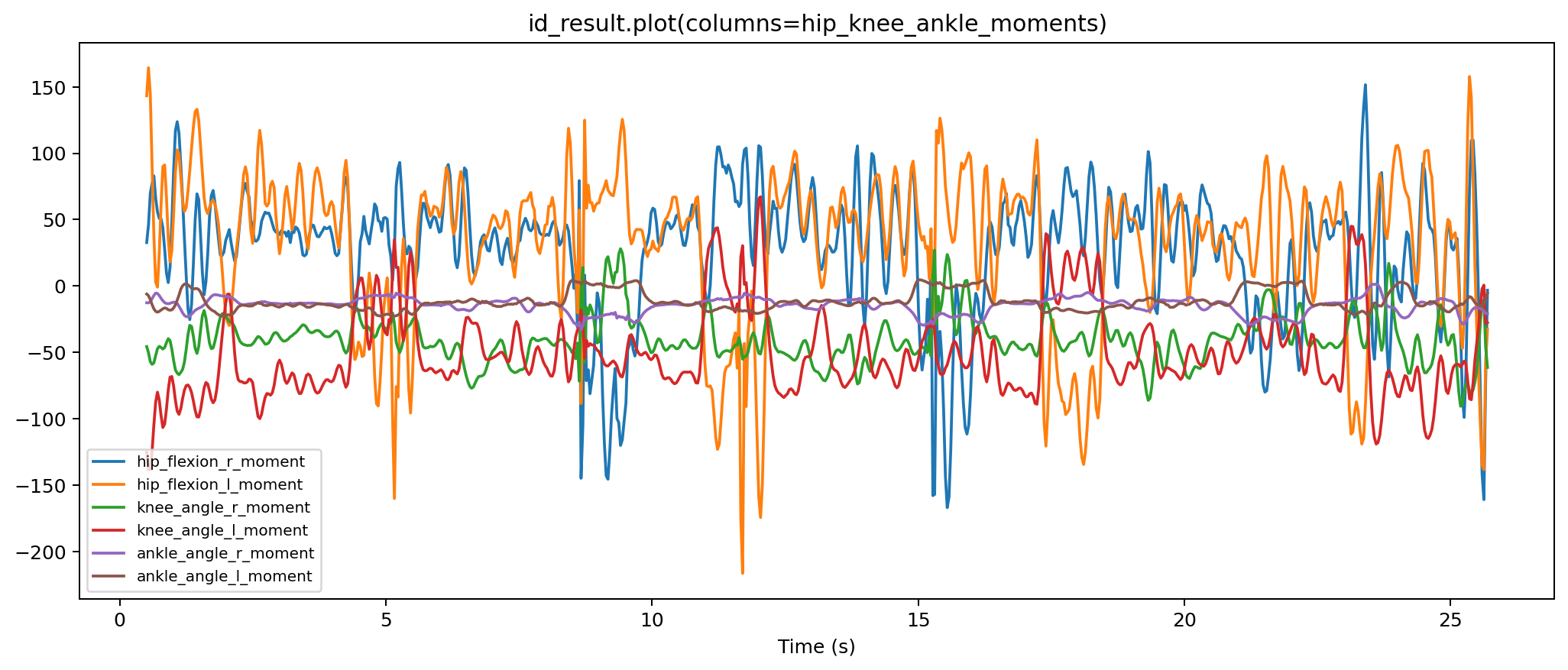
Inverse dynamics returns a .sto table. The sheet below is produced with id_result.plot(...) and highlights the main hip, knee, and ankle moments while the full table remains available through id_result.to_dataframe().

id_result = mm.run_id(
    ik=ik,
    external_forces=forces,
)

id_result.plot(columns=[
    "hip_flexion_r_moment", "hip_flexion_l_moment",
    "knee_angle_r_moment", "knee_angle_l_moment",
    "ankle_angle_r_moment", "ankle_angle_l_moment",
])
id_result.to_dataframe()

Stage 7: GLB Skeletal Animation Viewer

The GLB viewer shows the exported skeletal mesh animation in the same upload-first viewer used on the documentation site and by mm.glb_viewer().

viewer = mm.glb_viewer("outputs/subject01/visualizer/animation.glb")
viewer.show()

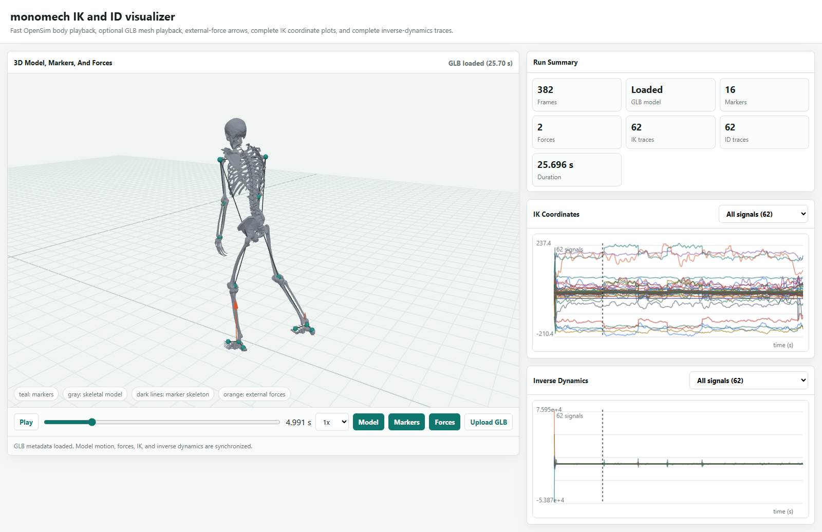
For synchronized marker fallback, force arrows, IK plots, and inverse-dynamics plots in one page, use the dashboard returned by mm.animate(...).

Output Checklist

Stage	Main output	What it tells you
2D pose	Pose2DResult stored in metadata	Whether image tracking is good enough to continue.
Root-centered 3D	Pose3DGlobalResult with root_centered=True	Body shape and relative joint motion before camera placement.
PnP global pose	Pose3DGlobalResult	Camera-placed, Y-up, floor-aligned marker trajectories.
TRC export	.trc	OpenSim marker input.
IK	.mot and StorageResult	OpenSim coordinate trajectories.
Estimated loads	ExternalLoads.xml and load .mot	Force vectors, application points, and torques over time.
ID	.sto and StorageResult	Generalized forces and moments.
Animation	.html and optional .glb	Synchronized model, markers, force arrows, IK, and ID review.