OpenSim Animation Export¶

monomech can export an animated OpenSim model to a single .glb file after inverse kinematics. The GLB contains the model geometry, the IK-driven animation, and optional inverse-dynamics metadata.

Use this when you want a portable file for review, presentation, web viewing, or sharing a quick motion result without opening the OpenSim GUI.

GLB skeletal viewer preview

Install¶

Animation export needs optional 3D dependencies:

python -m pip install "monomech[animation]"

This extra includes OpenSim bindings, pyvista, and pygltflib.

Basic Export¶

import monomech as mm

result = mm.save_opensim_animation(
    osim_path="outputs/subject01/scale/subject01_scaled.osim",
    mot_path="outputs/subject01/ik/subject01_ik.mot",
    out_glb_path="outputs/subject01/animation/subject01_motion.glb",
)

print(result.glb_path)
print(result.metadata["node_count"])

If geom_dir is omitted, monomech first uses its packaged full-body geometry, then looks next to the model for Geometry/, geometry/, and the model directory itself. Pass geom_dir only when using a custom model or mesh folder. For full-body models downloaded from zip archives, make sure this points at the real mesh folder, not a __MACOSX metadata folder. A good folder contains real .vtp, .obj, or .stl mesh files, not tiny ._name.vtp files.

IK And ID Together¶

Pass the inverse-dynamics output with id_path. The GLB animation is still driven by IK coordinates, while ID metadata is embedded in the file extras.

result = mm.save_opensim_animation(
    osim_path=scale.scaled_model_path,
    mot_path=ik.path,
    id_path=id_result.path,
    out_glb_path="outputs/subject01/animation/subject01_ik_id.glb",
)

print(result.metadata["id_summary"])

The GLB stays a single portable file, and the returned result keeps the export summary available in Python.

From A Full Pipeline¶

import monomech as mm

pose = mm.estimate_pose("data/subject01.mp4")
pose = mm.gap_fill(mm.smooth(pose))

scale = mm.run_scaling(
    pose,
    model="pose",
    output_dir="outputs/subject01/scale",
)

ik = mm.run_ik(scale, output_dir="outputs/subject01/ik")

loads = mm.estimate_grf(pose, body_mass_kg=75.0)

id_result = mm.run_id(
    ik=ik,
    external_forces=loads,
    output_dir="outputs/subject01/id",
)

animation = mm.animate(
    ik=ik,
    id=id_result,
    external_loads_path=id_result.metadata["external_loads_mot_path"],
    output_dir="outputs/subject01/visualizer",
    mode="balanced",
)
animation.show()

That is the complete review path: video in, pose tracking, OpenSim scale, IK, external loads, ID, and a browser-ready animated model out.

Geometry Folder Checklist¶

The GLB exporter uses the OpenSim model file for body transforms and the geometry folder for visual meshes. If the animation plays but the body is invisible or incomplete, check these first:

Check	What to do
Real mesh files are present	Open the folder and confirm files such as `r_pelvis.vtp`, `femur_r.vtp`, or similar are normal-sized files.
Avoid `__MACOSX` folders	Those folders usually contain `._*.vtp` metadata files and are not usable mesh geometry.
Match model and geometry family	Use the `Geometry/` folder that came with the `.osim` model whenever possible.
Packaged geometry	The default full-body meshes are included with `monomech`.
Pass `geom_dir` explicitly	Do this when using custom model geometry or a different mesh set.
Start with a preview export	Use `stride=3` and `decimate_target_reduction=0.5`, then lower those settings for final review.

Marker Positions¶

By default, the exporter also returns a DataFrame of model marker positions through time:

markers = animation.to_dataframe()
display(markers.head())

Disable this when you only need the GLB:

animation = mm.save_opensim_animation(
    osim_path=scale.scaled_model_path,
    mot_path=ik.path,
    out_glb_path="outputs/subject01/animation/subject01.glb",
    return_markers=False,
)

HTML Viewer¶

Write a lightweight local Three.js viewer for the GLB:

viewer = mm.glb_viewer(animation.glb_path)
viewer.show()

This writes the production viewer shell next to the GLB and references the GLB by path. The notebook displays the shell immediately, then the browser streams the GLB file. Use viewer.show(inline_glb=True) when the notebook browser cannot access the GLB path directly.

Open the upload-first base viewer with no model preloaded:

mm.glb_viewer().show()

Notebook IK/ID Dashboard¶

For notebooks and review sessions, use the fast visualizer first. It avoids GLB export and animates lightweight OpenSim body proxies directly from IK-driven body transforms:

viewer = mm.animate(
    ik=ik,
    id=id_result,
    external_loads_path=id_result.metadata["external_loads_mot_path"],
    output_dir="outputs/subject01/visualizer",
    render="fast",
)
viewer.show()

The fast viewer is the best default for checking motion, carried-load placement, ground-reaction arrows, IK coordinates, and inverse-dynamics traces during analysis. It controls body proxy meshes correctly, but it does not render the full anatomical surface meshes.

For very long trials, keep the browser payload small:

viewer = mm.animate(
    ik=ik,
    id=id_result,
    external_loads_path=id_result.metadata["external_loads_mot_path"],
    render="fast",
    max_frames=80,
    marker_stride=5,
)
viewer.show()

max_frames caps the number of frames displayed, and marker_stride can be raised when you want even faster OpenSim marker extraction.

For the fastest body-and-force preview, skip marker extraction and keep only major bodies:

viewer = mm.animate(
    ik=ik,
    id=id_result,
    external_loads_path=id_result.metadata["external_loads_mot_path"],
    render="fast",
    max_frames=40,
    include_markers=False,
    bodies="major",
    cache=True,
)
viewer.show()

cache=True stores the sampled OpenSim viewer data next to the HTML file. Re-running the same viewer with the same model, IK, ID, external loads, and speed settings reuses that cache instead of recomputing OpenSim body transforms.

Use the GLB path when you need the full model geometry:

viewer = mm.animate(
    ik=ik,
    id=id_result,
    external_loads_path=id_result.metadata["external_loads_mot_path"],
    output_dir="outputs/subject01/visualizer",
    render="glb",
    mode="balanced",
)
viewer.show()

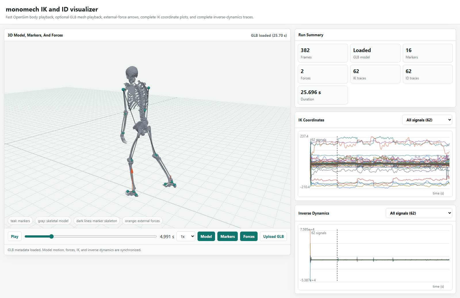
save_opensim_visualizer() creates the same Three.js HTML dashboard and can be paired with or without a GLB. It includes:

fast OpenSim body proxy playback
animated OpenSim GLB mesh playback when a GLB is provided
a 3D marker/skeleton fallback
external-force arrows from the generated external-load .mot
synchronized IK coordinate plots
inverse-dynamics trace plots
a browser-side Upload GLB control for GitHub Pages and notebook sharing

For carried objects and other body-local loads, pass both osim_path and ik_path when creating the visualizer. monomech uses the generated ExternalLoads.xml plus the IK motion to convert body-frame application points, such as hand_r, into ground coordinates before drawing the force arrows.

viewer = mm.save_opensim_visualizer(
    "outputs/subject01/animation/ik_id_viewer.html",
    osim_path=scale.scaled_model_path,
    ik_path=ik.path,
    id_path=id_result.path,
    external_loads_path=id_result.metadata["external_loads_mot_path"],
    glb_path=animation.glb_path,
    title="subject01 IK + ID",
)

viewer

In Jupyter, display the visualizer with one call:

mm.display_visualizer(viewer)

Pipeline results expose the same shortcut:

result.display()

When you already have IK and ID result objects from the staged API, animate() is the shortest path:

animation = mm.animate(
    ik=ik,
    id=id_result,
    external_loads_path=id_result.metadata["external_loads_mot_path"],
    output_dir="outputs/subject01/visualizer",
    render="fast",
    mode="preview",  # use "balanced" or "final" for higher quality
)

animation.show()

In a script, open viewer.html in a browser.

The same visualizer works well on GitHub Pages because it does not need a Python server. The online page lets readers upload their own .glb export directly in the browser:

In notebooks, viewer.show() displays the saved HTML through Jupyter's /files/ route when the output folder is under the notebook working directory. This is the fastest path because the browser streams the sibling .glb directly. If your notebook server cannot serve local files, use viewer.show(inline_glb=True) to display a patched in-memory copy that injects the GLB as a browser blob.

You can also build the dashboard without mesh geometry:

marker_df = mm.extract_opensim_marker_positions(
    osim_path=scale.scaled_model_path,
    mot_path=ik.path,
    stride=2,
)

viewer = mm.save_opensim_visualizer(
    "outputs/subject01/animation/marker_force_viewer.html",
    marker_dataframe=marker_df,
    ik_path=ik.path,
    id_path=id_result.path,
    external_loads_path=id_result.metadata["external_loads_mot_path"],
)

Open the online GLB visualizer

External Forces In The Viewer¶

When external_loads_path is provided, the dashboard reads the external-load .mot and displays force vectors as orange arrows in the 3D scene. The expected columns follow OpenSim-style force and point naming:

time right_vx right_vy right_vz right_px right_py right_pz

Each load needs velocity/force components ending in _vx, _vy, _vz and matching point columns ending in _px, _py, _pz. The viewer interpolates those vectors onto the displayed marker frames, scales the arrows for readability, and keeps them synchronized with the IK and ID plots.

For estimated ground-reaction forces from mm.external.estimate_grf(), monomech remaps pose axes into the same OpenSim-friendly coordinate system used by TRC export (X=z, Y=y, Z=x) and grounds the vertical axis before writing external loads. That keeps force application points aligned with the IK model rather than the original camera coordinate frame.

viewer = mm.save_opensim_visualizer(
    "outputs/subject01/animation/forces_viewer.html",
    marker_dataframe=animation.marker_dataframe,
    ik_path=ik.path,
    id_path=id_result.path,
    external_loads_path="outputs/subject01/id/subject01_external_loads.mot",
    glb_path=animation.glb_path,
)

File Size And Speed¶

mm.animate() has three production presets:

Mode	Use when
`mode="preview"`	Fast notebook review. Uses a larger stride and stronger mesh reduction.
`mode="balanced"`	Default. Good quality with practical notebook load times.
`mode="final"`	Highest fidelity. Uses every IK frame and no default decimation.

Override any preset directly:

viewer = mm.animate(
    ik=ik,
    id=id_result,
    mode="preview",
    stride=4,
    decimate_target_reduction=0.5,
    max_frames=160,
    embed_glb=False,
)

For direct GLB export, use these knobs when the file is too large or export takes too long:

Option	What it does
`stride=2`	Exports every second IK frame. Higher values make smaller files.
`thin_pos_tol=1e-4`	Removes translation keyframes that barely change.
`thin_rot_tol_deg=0.05`	Removes rotation keyframes that barely change.
`drop_static_nodes=False`	Keeps complete animation tracks for every exported mesh by default. Set to `True` for smaller review files.
`drop_origin_nodes=False`	Keeps every resolved mesh in the scene by default. Set to `True` only when diagnosing unresolved geometry sitting at the origin.
`decimate_target_reduction=0.35`	Reduces mesh triangle count before writing GLB.

The exporter caches repeated OpenSim frame transforms while baking. Full-body models often have several meshes attached to the same body, so this avoids asking OpenSim for the same body transform again and again within each frame.

For fast previews, start with:

animation = mm.save_opensim_animation(
    osim_path=scale.scaled_model_path,
    mot_path=ik.path,
    out_glb_path="outputs/subject01/animation/preview.glb",
    stride=3,
    decimate_target_reduction=0.5,
)

For final review, reduce or remove decimation and use stride=1.

Troubleshooting¶

Symptom	Fix
Missing optional dependency error	Install `python -m pip install "monomech[animation]"`.
No geometry is exported	Confirm the model uses compatible mesh names, or pass `geom_dir=` for a custom OpenSim geometry folder.
GLB contains unresolved parts at the origin	Try `drop_origin_nodes=True` for diagnostic exports, then inspect `result.metadata["missing_geometry"]` and the geometry folder path.
Animation looks too slow or too fast	Check the IK MOT time column and selected `t_start`, `t_end`, and `stride`.
File is too large	Increase `stride`, use keyframe thinning, or set `decimate_target_reduction`.